Intro to Google Colab and Jupyter Notebooks
Overview
In the previous lesson, you learned what data science is, what the field looks like in practice, and what this curriculum covers. Now it's time to set up the environment where all of your hands-on work will happen. In this lesson, you'll learn how to use Google Colab — a free, browser-based coding environment built on top of Jupyter Notebooks. You'll learn how to create and run notebooks, work with code and text cells, install libraries, and save your work. These are the mechanical skills that underpin every coding lesson in this curriculum.
Learning Objectives
By the end of this lesson, you will have learned how to:
- Set up and navigate Google Colab/Jupyter Notebooks.
- Execute code cells, manage notebook files, and install necessary libraries.
Key Terms
Jupyter Notebook: An interactive document format that combines live code, text, equations, and visualizations in a single file (.ipynb). The standard format for data science work.
Google Colab (Colaboratory): A free, cloud-hosted Jupyter Notebook environment provided by Google. Requires no local installation and includes free access to CPU and GPU compute.
Cell: The basic unit of a notebook. Each cell is either a code cell (runs Python) or a markdown cell (displays formatted text).
Kernel: The computational engine that executes the code in a notebook. In Colab, the kernel runs on a Google server. "Restarting the kernel" clears all variables and resets the runtime.
Runtime: Colab's term for the virtual machine and kernel assigned to your session. Runtimes disconnect after a period of inactivity.
Markdown: A lightweight markup language for formatting text using simple symbols (e.g., **bold**, # Heading, - bullet).
Magic command: A special Jupyter command prefixed with ! or % that interacts with the shell or notebook environment rather than executing Python (e.g., !pip install pandas).
Introduction
Every lesson in this curriculum has a companion notebook hosted in Google Colab. When you click a "Colaboratory notebook" link in any lesson, it opens a pre-configured notebook where you can run the lesson's code, modify it, and experiment freely.
Google Colab is free to use, requires no installation, and runs entirely in your browser. The only requirement is a Google account.
Opening Google Colab
Navigate to colab.research.google.com. You'll see a welcome dialog with options to:
- Open a recent notebook
- Open from Google Drive
- Open from GitHub
- Create a new notebook
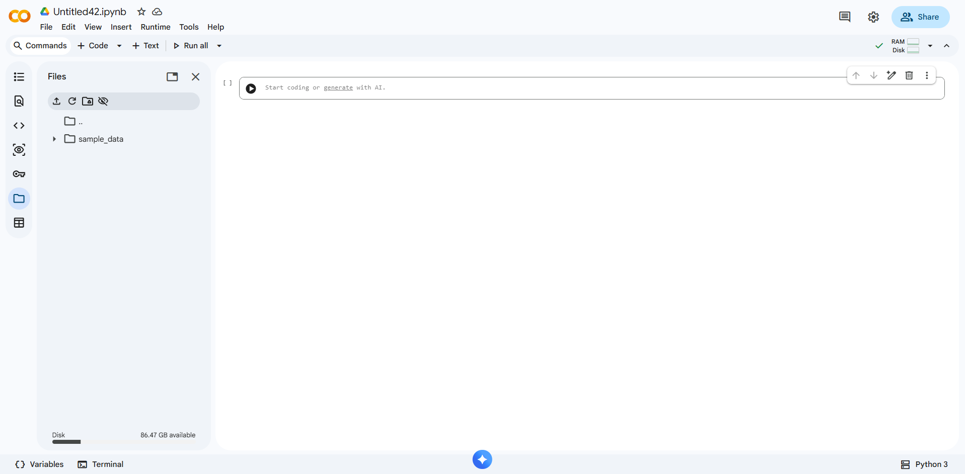
Select New notebook to create a blank notebook. A new tab will open with a single empty code cell.
The Notebook Interface
A Colab notebook has three main areas:
┌─────────────────────────────────────────────────┐
│  File  Edit  View  Insert  Runtime  Tools  Help │  ← Menu bar
├──────┬──────────────────────────────────────────┤
│      │  + Code   + Text                         │  ← Add cell buttons
│ File │  ─────────────────────────────────────── │
│  Nav │  [ ] Code cell                           │  ← Active cell
│      │                                          │
│      │  [ ] Code cell                           │
│      │                                          │
│      │  ─── Markdown cell ───────────────────── │
└──────┴──────────────────────────────────────────┘
- Menu bar: File operations, runtime control, settings
- + Code / + Text: Add a new code or markdown cell below the selected cell
- Cells: The content area where you write and run code or formatted text
Code Cells
A code cell runs Python. Click inside a cell and type Python code:
print("Hello, data science!")
2 + 2
Run a cell by:
- Pressing Shift + Enter (runs and moves to the next cell)
- Pressing Ctrl + Enter (runs and stays on the same cell)
- Clicking the ▶ play button to the left of the cell
Output appears directly below the cell:
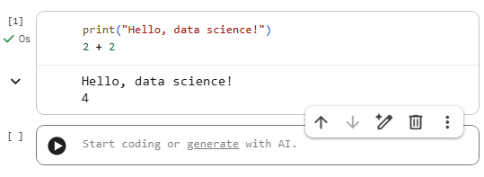
The last expression in a cell is displayed as output automatically — you don't need print() for simple values.
Markdown Cells
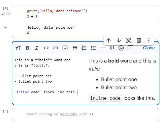
A markdown cell displays formatted text — headings, bullet points, bold, code snippets, and mathematical formulas. Double-click any markdown cell to edit it.
# This is a heading

This is a **bold** word and this is *italic*.

- Bullet point one
- Bullet point two

`inline code` looks like this.
Shift + Enter renders the markdown. Markdown cells are used for section titles, explanations, and documentation — a well-organized notebook alternates code and markdown to tell a story.
Essential Keyboard Shortcuts
| Action | Shortcut |
|---|---|
| Run current cell | Shift + Enter |
| Run cell, stay on cell | Ctrl + Enter |
| Add code cell below | Ctrl + M, B |
| Add code cell above | Ctrl + M, A |
| Delete selected cell | Ctrl + M, D |
| Switch cell to Markdown | Ctrl + M, M |
| Switch cell to Code | Ctrl + M, Y |
| Comment/uncomment | Ctrl + / |
| Undo | Ctrl + Z |
Variable Persistence
Variables defined in one cell are available in all subsequent cells — they persist in the kernel's memory for the entire session:
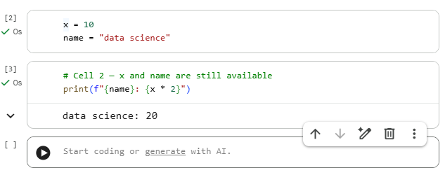
Important: Cells can be run in any order, and variables reflect the last time each cell was executed — not the order they appear on screen. Always run cells top-to-bottom when starting fresh to avoid confusion.
Restarting the Runtime
If something goes wrong — variables are in an unexpected state, a library import failed, or memory is full — restart the kernel to get a clean slate:
- Runtime → Restart runtime (clears all variables, keeps notebook content)
- Runtime → Restart and run all (clears variables and reruns every cell from top to bottom)
After a restart, you must rerun all cells from the beginning.
Installing Libraries
Colab comes with many data science libraries pre-installed (pandas, numpy, matplotlib, seaborn, scikit-learn). If you need a library that isn't included, install it with !pip install:
!pip install plotly
The ! prefix runs a shell command rather than Python. The installation applies only to the current runtime session — if the runtime restarts, you'll need to install again.
Check which version of a library is installed:
import pandas as pd
print(pd.__version__)
Mounting Google Drive
By default, Colab notebooks cannot access files on your Google Drive. To read or write files (like CSV datasets), mount your Drive:
from google.colab import drive
drive.mount("/content/drive")
A pop-up will ask you to authorize access. After mounting, your Drive is accessible at /content/drive/My Drive/:
import pandas as pd

# Read a CSV from Google Drive
df = pd.read_csv("/content/drive/My Drive/my_dataset.csv")
print(df.head())
Uploading Files Directly
For quick uploads without mounting Drive, use the built-in file picker:
from google.colab import files

uploaded = files.upload()   # Opens a file picker dialog
After uploading, the file is accessible by name in the current session:
import pandas as pd
df = pd.read_csv("my_dataset.csv")
Saving Your Notebook
Colab autosaves to Google Drive. You can also save manually:
- File → Save (
Ctrl + S) — saves to Drive - File → Download → Download .ipynb — saves a local copy of the notebook file
- File → Save a copy in GitHub — pushes the notebook directly to a GitHub repository (covered in the next lesson)
Notebooks are saved as .ipynb files — JSON documents that store your code, outputs, and markdown together.
Checking Your Setup
Run the following cell to confirm that the core libraries are available and print their versions:
import sys
import pandas as pd
import numpy as np
import matplotlib
import sklearn

print(f"Python:      {sys.version.split()[0]}")
print(f"pandas:      {pd.__version__}")
print(f"numpy:       {np.__version__}")
print(f"matplotlib:  {matplotlib.__version__}")
print(f"scikit-learn:{sklearn.__version__}")
If all five lines print without error, your environment is ready.
Conclusion
Google Colab is the environment you'll use for every hands-on exercise in this curriculum. You now know how to create and run notebooks, work with code and markdown cells, install libraries, load files, and save your work. These are the mechanical foundations — get comfortable with them early, and they'll become second nature. In the next lesson, you'll learn how to use GitHub to save, version, and share your notebooks.